Renders as Ground Truth: Training a Segmenter on 40,000 Synthetic Images
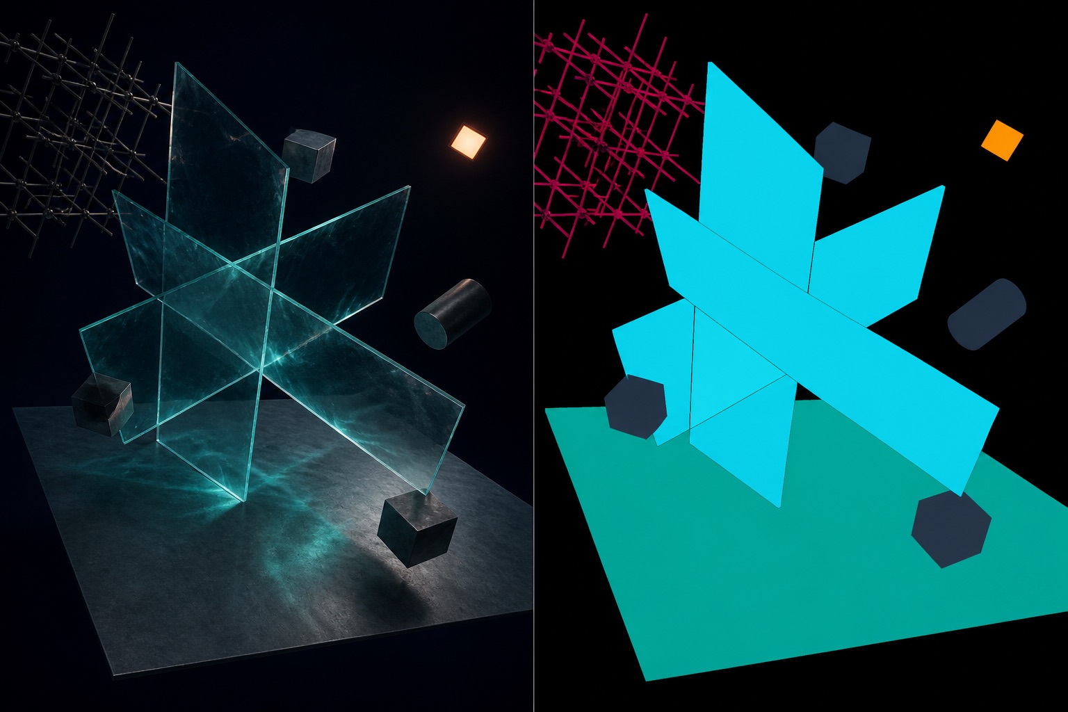
Dense per-pixel labels are the most expensive annotation a computer-vision project can ask for. A bounding box is four clicks; a polygon around one object is thirty. A complete pixel-accurate partition of a scene into regions — every pixel of a surface belonging to that surface, including the parts seen through glazing, behind a wire mesh, at grazing angles under blown-out sunlight — is an hour of skilled labour per image, and two annotators will disagree on the boundary.
A renderer already knows the answer. Computing which surface every ray hit is what rendering is. Persuade it to write that knowledge out as an image instead of a photograph and the labels stop being an annotation problem and become a rendering problem, solved once in code and then run ten thousand times overnight.
The system described here took that trade to production. It segments a large planar surface out of a single camera frame, was trained on nothing but renders of a synthetic facility, and reaches 0.9950 IoU on the target region and 0.9973 pixel accuracy on held-out synthetic data. Tested afterwards on real photographs it lands at 97-99% pixel accuracy — one to three points below the synthetic figure, across a domain change that usually costs far more than that. No fine-tuning on real data, no domain adaptation, no style transfer.
That transfer did not arrive automatically. Two configurations of the same pipeline failed to transfer at all, and one decision about the label ontology is what made the shipped one work.
What follows starts with a primer on the 3D vocabulary the rest depends on. If you already build scenes for a living, skip to the scene section.
What 3D rendering is, and why it can label an image
Everything below depends on a handful of ideas from 3D graphics that have no counterpart in a normal machine-learning workflow. If your background is computer vision and you have never opened a 3D package, this is the vocabulary the article assumes.
A scene is geometry, materials, lights and a camera
Geometry is surfaces described as meshes: lists of vertices joined into triangles or quads. A mesh on its own is just data; placing it in the world with a position, rotation and scale makes it an object. A scene is a tree of such objects.
One subtlety matters later. Packages let many objects share a single mesh — instancing — so a facility with four identical units can hold four objects backed by one copy of the geometry. That saves enormous memory, and it is also an excellent way to corrupt your labels.
A material (or shader) says what a surface does to light. Modern packages express this as a BSDF, a bidirectional scattering distribution function, configured by a handful of physically meaningful parameters. Four appear repeatedly below. Base colour is the surface’s own colour, and for a metal it doubles as the reflectance. Roughness controls how tightly reflections focus: 0 is a mirror, 1 is chalk. Transmission makes a surface pass light through it, which is how glass is made. Emission makes a surface a light source in its own right, radiating a flat colour that no lamp in the scene affects. That last property is the one this entire pipeline is built on.
Lighting can come from modelled lamps, or from an HDRI environment map: a single high-dynamic-range photograph, stored in equirectangular projection so it wraps the scene as a sphere, that serves simultaneously as the visible backdrop and as the only light source. One file gives you a sky, a horizon, a sun in the right place and physically consistent bounce light. Swapping the file relights the whole scene, which is why it becomes a sweep axis.
A camera is defined much like a real one: a focal length and a sensor size, which together fix the field of view, plus a projection model. Rectilinear projection keeps straight lines straight and is what a normal lens does. Fisheye projections trade that for a much wider field of view, and they matter here because many wide and ultrawide lenses are fisheyes rather than rectilinear. If the deployed camera barrel-distorts, the training data has to as well.
Rendering is simulating light until you have a pixel
The dominant technique for realism is path tracing. For each pixel the renderer shoots rays out through the camera, follows them as they bounce off surfaces, and accumulates the light that arrives. One ray gives a wildly noisy estimate, so the renderer averages many — the samples per pixel count, usually written spp. Noise falls as samples rise, and cost rises linearly with them, which makes spp the main quality-versus-time dial. Because high sample counts are expensive, renderers ship denoisers that clean up a low-sample image statistically, letting you use far fewer.
Two more settings appear repeatedly below. The pixel filter decides how the several sub-pixel samples inside one pixel are weighted together; widening it blends across pixel boundaries, which is anti-aliasing, the soft edge that makes a rendered image look smooth. And a view transform with an exposure control maps the renderer’s unbounded physical light values into the 0-255 range a file can hold, exactly as a camera’s tonemapping does.
The photographic output — path traced, denoised, anti-aliased, tonemapped — is conventionally called the beauty render, to distinguish it from the renderer’s other outputs.
Render passes: the outputs that are already label-shaped
A renderer does not only produce a picture. In the course of tracing a ray it necessarily determines the distance to the surface it hit, that surface’s orientation, which object it belonged to, and which material was on it. Most renderers will write any of these out as a separate image aligned pixel-for-pixel with the beauty render — a render pass. Depth passes, normal passes, material-index passes and object-identity passes (Blender calls its version Cryptomatte) are standard features, built for compositors who want to relight or mask a shot after the fact.
Look at that list from a machine-learning angle and the significance is hard to miss. A depth pass is a depth map, and an object-identity pass is an instance segmentation mask. They are exact, noise-free, and perfectly registered to the image, because the same ray query that produced the pixel produced them. No annotator, no registration step, no disagreement about the boundary.
This pipeline uses a variant of the idea rather than the built-in passes. Instead of asking the renderer for an identity pass, it temporarily replaces every material in the scene with a flat emission shader of a known colour and renders normally, then recovers the classes by matching pixel colours back to those references. The result is equivalent, and it buys two things: the mapping from colour to class lives in the script rather than in a compositor graph, and arbitrary label semantics become expressible — including regions that correspond to no object at all, which the built-in passes cannot represent.
The tools
The work here was done in Blender, which is free and open source, ships a production path tracer called Cycles and a much faster real-time rasteriser called EEVEE, and exposes essentially its entire feature set through a Python API. A script can build geometry, rewrite materials, place cameras, trigger renders and read pixels back, and the whole thing runs headless on a server with no display attached. That combination is why a 3D package ends up inside a machine-learning pipeline: it scripts like infrastructure and happens to also have a GUI.
It is not the only option. Game engines such as Unreal and Unity are used the same way, and there are frameworks built specifically for this job — BlenderProc and Kubric wrap Blender for dataset generation, NVIDIA’s Omniverse Replicator and Unity’s Perception package do the same in their own ecosystems. They handle much of what the following sections describe by hand. This project went bespoke for two reasons: the scene was hand-assembled by an artist rather than composed from a catalogue, and several of the label classes were domain-specific rules rather than objects. A general framework is not shaped for either. If your scene is procedural and your labels are ordinary object masks, start with a framework.
| Term | Meaning |
|---|---|
| mesh | a surface as vertices and faces; the geometry itself, independent of where it sits |
| instancing | several objects sharing one copy of a mesh — cheap in memory, dangerous for per-object labels |
| BSDF | the function describing how a surface scatters light; the thing a material configures |
| emission shader | a material that radiates a fixed colour regardless of scene lighting |
| transmission | the BSDF parameter that lets light pass through a surface; how glass is made |
| path tracing | rendering by tracing many light paths per pixel and averaging them |
| spp | samples per pixel; the noise-versus-time dial |
| denoising | statistical cleanup of a low-sample render, so fewer samples suffice |
| pixel filter | how sub-pixel samples combine into one pixel; widening it is anti-aliasing |
| view transform / exposure | the mapping from physical light values to displayable pixel values |
| beauty render | the photographic output, as opposed to a data pass |
| render pass | an auxiliary output aligned to the beauty render — depth, normals, object identity |
| Cryptomatte | Blender’s per-object identity pass; an instance mask by another name |
| HDRI | a high-dynamic-range equirectangular photograph used as both backdrop and light source |
| rectilinear / fisheye | camera projection models: straight lines preserved, versus a much wider barrel-distorted field of view |
| headless | running the package as a batch process with no GUI, which is how a sweep runs on a server |
The scene is an artifact, not a script
The instinct of an engineer approaching synthetic data is to generate the world procedurally: parameterise everything, commit the generator, treat the scene as build output. That instinct is right about the sweep and wrong about the scene.
The environment here is a facility built from repeated enclosed units — a large flat ground surface per unit, glazed side and end panels, wire mesh above them, overhead floodlights, people, vegetation, street furniture. It was assembled interactively, by hand, in the Blender UI. There is no build script for it. The 191 MB scene file is the source of truth, and if it is lost the only survivors are the renders. That is documented in exactly those terms, because pretending otherwise is how a team discovers at the worst possible moment that its most valuable asset was never reproducible.
What is scripted is everything downstream: the sweep, the render passes, the mask decode, the dataset build. The seam between the two is a naming contract. The sweep does not know what a unit is; it knows the ground object of unit rXcY is named Floor__rXcY, that each glazed panel carries a custom property holding its own stable id, that the unit’s surface material is Grass floor rXcY. Every address into the geometry travels through that convention, which is what let a second scene variant drop straight in. That variant was script-built from a purchased asset with a structural frame the first one lacked, and the script’s entire job was to rename, split and tag nine monolithic imported meshes until they satisfied the same contract. The sweep then rendered both scenes without knowing they differed. It classified the split panels by position rather than by import order, since import order is an artefact of whoever exported the file and would silently reshuffle on re-export.
Fix the physics before you sweep. Three shipped asset materials were physically wrong in ways only real lighting reveals, and all three were caught by looking at renders rather than by reading the file. The metalwork was base colour (0,0,0) with Metallic=1 — for a metallic BSDF the base colour is the reflectance, so pure black returns no light at any angle, leaving a void where steel should be. The ground surface at roughness 0.45 read as brushed metal, and from one camera position the sun’s mirror direction blew out 60% of the near floor. Glazing at roughness 0.03 under full transmission came out 3.3× softer than at 0.0, since every refracted ray scatters and each crosses two interfaces. A sweep launched before these were fixed bakes a systematic defect into thousands of images.
Turning a renderer into a label generator
The mechanism states in one sentence and contains enough traps to justify several. Render the scene twice from the same camera, once for the picture and once for the labels, with everything that makes a picture look good switched off for the second pass. The label passes share the beauty pass’s camera exactly, which is the whole reason the approach works: alignment is not approximated, it is identical by construction. Three lightings per pose then amortise one mask set across three training images.
Everything that helps a photograph hurts a label
For a mask pass, every material becomes a flat emission shader of a known colour, environment light drops to zero strength, exposure is forced to zero, samples fall from 96 to 16, denoising goes off, and — the one people forget — the pixel filter width goes to nearly zero. Anti-aliasing is a feature in a photograph and a defect in a label: it invents intermediate colours along every edge that belong to no class. Denoising is worse, because it invents them non-locally.
Classes are then encoded as colour and recovered by nearest-reference matching with a tolerance, in the same encoding the renderer wrote. Anything further than the tolerance from every reference becomes background rather than being forced into the nearest class. For a pixel the pass cannot account for, background is the honest answer.
Labels can come from scene knowledge, not just from surfaces
Two of the candidate label classes correspond to no object in the scene at all. The ground surface was subdivided into sub-regions by placing thin emissive rectangles at floor level, sized from the ground object’s bounding box and known real-world dimensions, and rendering those. Painted markings were extracted by recolouring one material slot on the ground object white and everything else black.
This generalises further than anything else in the pipeline. A renderer will label anything you can express geometrically — a region defined by a rule, a distance band, a projected footprint, an occlusion relationship — whether or not it corresponds to something an annotator could see and outline. Some of the most useful labels are ones a human physically could not produce.
Trap: instanced geometry shares its mesh. The units were instanced by copying objects, which shares the underlying mesh data: 72 glazed panels over 18 meshes, one mesh-fence object across four units. Assigning a mask material at the mesh level therefore repaints every copy at once. The target unit’s masks came out containing the other three units, seen through the glazing: 91.8% of frame before the fix, 14.7% after, with fragmented masks going from 15 of 33 to zero. The fix is one line. Write the material as an object-level override so it stays on that object alone, and restore by dropping the override rather than reassigning by index. Diagnose it by colouring “ours” and “everything else” differently and counting pixels; if “ours” is 0%, the shared-data write is the cause.
Amodal by choice, and stated as such
People, foreground fixtures and vegetation are hidden during every mask pass, so the surface label extends through the legs of anyone standing on it. That is correct if the question is “where is the surface” and wrong if it is “what is visible”. The point is that it is written into the model’s own documentation as a property of the labels rather than left to be discovered. A renderer makes both variants nearly free; this project shipped only the amodal one, deliberately.
One related mechanic: the fisheye lenses were rendered oversized and centre-cropped, with the crop applied to the beauty render and every mask by the same code path. Any geometric post-process that reaches image and label separately will drift them apart, invisibly, until a model refuses to converge.
Sweeping the space that reality varies
The sweep is where a synthetic dataset earns or loses its value, and the discipline is separating two kinds of axis. Geometric axes change what the camera sees and must be crossed, because their combinations are not interchangeable: a low mount with a wide lens frames nothing like a high mount with a narrow one. Appearance axes change how the same geometry looks, and can be sampled, because they are independent of the framing and of each other. Sampling them per image rather than crossing them is domain randomization: instead of trying to match reality’s appearance, you span a range wide enough that reality falls inside it, and the model learns to ignore the axis entirely.
The crossed axes, and what they multiply to
| Geometric axis | Values | Count |
|---|---|---|
| unit in the facility | 2 rows × 3 columns, one of the columns structurally different | 6 |
| mounting wall | either end of the unit — mirrors the whole labelling convention | 2 |
| lateral position | centre, off-centre, corner | 3 |
| mount height | 0.5 · 1.0 · 1.5 · 2.0 · 2.5 · 4.0 m | 6 |
| lens | ultrawide fisheye · rectilinear · 155° fisheye | 3 |
| standoff from the mounting plane | 0.2 m behind the glazing · 1.0 m behind it · 0.2 m inside the volume | 2 of 3 |
| yaw offset | −15° · 0° · +15° from the base aim | 3 |
| pitch offset | −10° · 0° · +10° | 3 |
| distinct camera poses after feasibility gates | 6,642 | |
| lighting environments drawn per pose | 3 sampled from 28 available | ×3 |
| training images, default configuration | 19,926 |
The raw cross product is larger than 6,642; gates cut it down. The 4 m mount renders only at the centre lateral position, because off-centre at that height the frame fills with near mesh. The 1.0 m standoff exists to put a structural frame between lens and glazing, so it gets a three-rung height ladder rather than the full six, and it is refused outright on any wall with a neighbouring unit 0.4 m behind it, which would stand the lens inside the neighbour. Roll is not swept at all.
Lighting is the other multiplier: 17 HDRI environments, each rendered with and without vegetation where that makes sense (six are interiors, where a tree canopy does not), giving 28 distinct lighting conditions. Enabling the third standoff would take the pose count to 11,826; enumerating all 28 lightings on every pose rather than sampling three would take the image count to 331,128. An offline mirror pass, needed only for a chirally-defined class set, doubles it again.
Why lighting is sampled and geometry is crossed. Rendering every lighting on every pose is redundant: the geometry is identical, so the whole mask set is shared across a pose’s lightings and only the beauty render is recomputed. Three random draws per pose cover the same lighting space 9× more cheaply, and across thousands of poses each environment still recurs hundreds of times. The appearance axes go further: surface colour (5 palettes), wall colour and material (5 plus a glazed/opaque mode), fixture colour (2), metalwork colour (6), environment rotation, exposure and sub-degree camera jitter are all drawn per pose from its seed rather than crossed. Crossing them instead would give 11,826 × 28 × 5 × 6 × 2 ≈ 19.9 million images — thousands of GPU-days for coverage that random sampling reaches in one night, because those factors are independent and the model needs their marginals, not their joint.
What was actually rendered, and where it saturated. The shipped corpus was not the ceiling. Combining both scene variants and both the glazed and solid-wall configurations, the sweep produced roughly 40,000 images: an order of magnitude below the 331,128 the lighting axis alone could have supplied, and three orders below the full appearance cross product. That was enough. It covered the variety of the real cases the model had to handle, and it is the corpus behind the transfer result below; nothing in the real-photograph evaluation pointed at a gap more rendering would close. The value of enumerating the axes is not that you render all of them. It is that you know exactly what you are choosing not to render, and can go back for one specific axis when a gap does show up.
Two more reductions transfer to any sweep. Five lateral positions collapse to three, because positions 4 and 5 are exact horizontal mirrors of 2 and 1 — a 40% cut at zero information cost for any achiral class set, and recoverable by the offline mirror pass if the class set is chiral. And the environment classification itself was measured rather than assumed: each HDRI’s artificial-lighting and interior flags come from measured sky radiance over the upper hemisphere of the equirectangular map, not from its filename, with each class’s exposure target calibrated against percentile statistics of the rendered frames rather than by eye.
For scale: at roughly 46 s of wall time per pose, the 6,642-pose configuration is about 86 process-hours, or one overnight run at four-way concurrency on a 32-core box. That is the number that makes the whole approach viable, and it is why pruning axes matters more than buying hardware.
Determinism per sample, not per run. Every random choice in a pose — camera jitter, environment rotation, exposure wobble, which colours the appearance axes take — comes from a seed hashed from that pose’s own identifier. Same pose, same result, on any machine. Two related bugs are worth naming. The appearance colours were originally resolved once per process, so a 3,456-pose run came out with a single fixture colour: technically random, useless as variation. And the seed needs a stable hash, not the language’s built-in one, which is salted per process and would re-randomise everything across runs of the same seed.
Finally, the per-pose metadata file is written last, so its presence means the pose completed. A multi-day render will be interrupted by a reboot, a dropped connection or a full disk, and that one ordering choice is what makes it restartable without redoing finished work. The cost profile also surprised everyone: the pipeline was CPU-bound, not GPU-bound. Per pose, roughly 8 s of mask rendering, 8.5 s of CPU mask post-processing and 30 s of beauty renders, with the GPU at 25% while load average hit 56 on 32 cores. The hot spot was the nearest-colour decode. More GPU would have bought nothing.
From renders to a dataset
Raw passes are not a dataset. Three transformations sit between, and each encodes a decision.
Welding. A wall built from adjacent panels, photographed through a wire mesh, decodes into hundreds of slivers: the frame between panels is a 1-3 px seam and the mesh wires punch holes through everything. A morphological closing at a radius measured against those seams, then hole filling, then dropping components below 1% of the largest, turns each composite into one solid region. The radius is small on purpose, because a large kernel would also bridge genuinely disjoint things, like a wall and its reflection a thousand pixels away.
The class set is a build parameter. Six regions could be labelled from the passes. Which of them become classes is a flag on the dataset builder, and everything downstream — trainer, exported metadata, consuming SDK — reads the class list from the data rather than hard-coding it. That is what made it cheap to narrow the ontology twice, which turned out to be the decision the whole result rested on.
Split by generative parameter, not by file. Train, validation and test split by camera position: every orientation and lighting of one physical placement lands in the same split, assigned by a deterministic hash of the position key so rebuilds are stable. Split per image instead and validation is scored on ±15° near-duplicates of training frames, which inflates the number and destroys its diagnostic value. In a synthetic dataset the generative parameters are the correct unit of independence, and you know them exactly.
Two practical notes. JPEG encoding shrank the payload roughly sevenfold, 19 GB to 2.8 GB, at no measurable cost since training downscales on load anyway. And the builder exits non-zero if any pose failed, because a partially-built dataset is usable, plausible and wrong.
Training, and the one augmentation that inverts the label
The model is SegFormer-B2: NVIDIA’s Mix Transformer encoder (MiT-B2, published as nvidia/mit-b2), hierarchical so it emits features at four scales, under a deliberately lightweight all-MLP decode head. Fine-tuned from its ImageNet weights at 1024×640, batch 8, learning rate 6e-5 on a one-cycle schedule, cross-entropy plus 0.5× soft multiclass Dice. Fifteen epochs, 5.6 minutes each on one 24 GB consumer GPU, 22.3 GB peak. The Dice term earns its place when a class is a small share of pixels: in the two-class configuration the thin wall region was 8.7% of labelled pixels against the ground surface’s 91%.
Two constraints set the input resolution. The renders’ own resolution is the ceiling, since there is no information above it, and VRAM is the practical bound: 1024×640 was the largest input fitting at batch 8 while holding the renders’ exact aspect. SegFormer accepts any input size, because position information comes from a depthwise convolution in its feed-forward blocks rather than from fixed positional embeddings. That flexibility is a trap, addressed below.
Augmentation is the sim2real lever, and it is the photometric half that matters. Geometric jitter — small affine scale, translate, rotate — helps in the ordinary way. Brightness and contrast at ±0.28, gamma 0.70-1.40, hue and saturation shifts, motion and Gaussian blur, and JPEG compression at quality 45-95 do something different: they stop the model keying on the renderer’s exact tonemap, which no real camera will reproduce. This is the photometric half of domain randomization, and it is the whole sim-to-real strategy. No adversarial alignment, no feature matching, no paired data. If one setting deserves the credit for the transfer result below, it is this one.
Trap: chiral classes cannot be flipped. Four of the six candidate classes were defined relative to the camera — the wall on its left, the wall on its right — so a horizontal flip changes the correct answer. Mirroring pixels while keeping the label teaches the model to be mirror-invariant, which is precisely to ignore the cue the class encodes; at flip probability 1.0 it learns the labels exactly inverted. The correct treatment is to turn the online flip off and generate mirrored copies offline with the class pairs swapped, keeping each mirror in its source split since a mirror is a near-duplicate of its original. Offline mirroring reached a previous run’s 21-epoch peak in 12 epochs. The pipeline now refuses to start if a chiral class is selected with flipping on, and refuses to mirror a chiral class whose partner is absent from the set. The surviving classes are achiral, so the shipped model flips freely and for free.
The quality reached, in simulation and in reality
On a held-out test split of 1,518 images, split by camera position:
| Metric | Value |
|---|---|
| background IoU | 0.9939 |
| target region IoU | 0.9950 |
| mIoU | 0.9945 |
| pixel accuracy | 0.9973 |
| validation mIoU (best epoch) | 0.9946 |
Validation 0.9946 against test 0.9945, so no gap: the split holds and the model converged. Taken alone that is a convergence check and nothing more, because validation and test differ from training only in camera position, with the same scene, assets, renderer and lighting library behind all three.
The transfer result. Tested afterwards on real photographs — real cameras, real sites, surface colours and materials the scene never contained, shot through dirty glazing with reflections, day and night — pixel accuracy came in at 97-99%, against 0.9973 on the synthetic test above. A one-to-three-point drop is close to the measurement floor for this kind of comparison, and far less than a domain change of this size normally costs. No fine-tuning on real data, no domain-adaptation stage, no style transfer. A renderer, a sweep and a photometric augmentation policy were enough.
That is the headline, and it was not a foregone conclusion. The same pipeline produced two configurations that did not transfer and one artifact class that persisted. All three were found by looking at real photographs, and none of them was visible in any synthetic metric.
What transferred, and what did not
The ontology started at six candidate regions and shipped with one. That narrowing is the decision the transfer rests on, and the pattern in it is general.
The region that transferred is large, contiguous, geometrically grounded, and defined by its own appearance: a ground plane with a characteristic material, always in a predictable part of the frame. Its boundaries came out accurate on surface colours the training set never contained.
The regions that did not were defined by relationship rather than by appearance: “the wall on the camera’s left”, “the wall on its right”. On real photographs those classes attached to the neighbouring unit entirely outside the one being photographed, and to the trees behind it. The cause is structural. Every synthetic pose saw three other units through the glazing in one fixed grid arrangement, so “adjacent structure” correlated perfectly with the side-wall classes. An earlier model scoring 0.959 box mAP50-95 on synthetic test had exactly this failure. No synthetic metric can detect it, because the confound sits identically in train, validation and test.
The general rule is harsher than it sounds: anything held constant across your whole synthetic corpus is invisible to every metric computed on that corpus, and free for the model to use as a shortcut. A class whose definition depends on that constant will not transfer. A class defined by its own appearance and geometry will. List your constants explicitly, treat that list as your risk register, and expect the ontology to narrow toward the classes that do not lean on them. Dropping the wall class did cost a downstream capability, and that cost is recorded next to the numbers rather than quietly absorbed.
The one artifact that persisted, and the resolution trade behind it
Training at 1024×640 instead of 512×320 improved every synthetic metric, and made a specific sub-percent real-photograph artifact several times more frequent: the target class predicted in a small region disconnected from the surface, mostly overcast sky.
| Measure | 512×320 | 1024×640 |
|---|---|---|
| target IoU (synthetic) | 0.9894 | 0.9936 |
| thin-region IoU (synthetic) | 0.9565 | 0.9790 |
| mIoU (synthetic) | 0.9764 | 0.9875 |
| stray area, 92 real photos | 0.173% | 0.945% |
That mechanism inverts the usual intuition about resolution. At 1024 the model resolves real-world fine texture — grain, dirt, mesh moiré, cloud structure — that the renders never contained. Downscaling to 512 had been acting as a low-pass filter that hid that part of the domain gap. The higher-resolution model is genuinely better at the synthetic task and genuinely more exposed to reality, and no synthetic metric can show you the trade: every number in the left-hand column says the larger input is strictly better.
The mitigation is a post-process, and it was deliberately kept out of the model. The target region is always the component touching the bottom of the frame, so keeping only that component removes every observed stray. Putting it in the model path would have made the raw metric less honest.
A negative result that was predictable from the training config. Nine OpenCV pre-processing variants were tested at inference — CLAHE at two clip limits, gamma up and down, unsharp masking, white balance, detail enhancement — on all 92 real photographs, motivated by dark reflective glazing. Every one was neutral or worse, with per-image effects of inconsistent sign, which is the signature of noise. The reason is in the training config: those transforms land inside the invariance the augmentation already built, so applying them at inference is close to a no-op by construction. If your augmentation spans a transform, that transform cannot be your fix. The lever is training data or resolution.
One caveat stays true regardless. The synthetic numbers are computed against exact labels, and the real-photograph figure is a measurement on a modest set. A permanent hand-labelled real evaluation set of even 15-20 images turns every question of this kind from an argument into a measurement, and is worth more than another week of rendering. Budget for it on day one.
Shipping: the export is a gate, not a report
The trained checkpoint becomes an ONNX graph plus a generated metadata sidecar, and the export fails rather than warns if the argmax disagrees with the source model on a single pixel; if the graph is not self-contained (the exporter’s default spills weights into a sibling file a byte-embedding consumer cannot follow); or if the opset read back from the written file differs from the one requested, which happens silently when an operator has no adapter below a given version.
The sidecar carries the class map, required input scale, normalisation constants, measured scores and caveats, and every derivable field comes from the checkpoint’s own config, the run’s arguments and its metrics file. The normalisation constants are imported from the training module rather than restated, because they are the one thing that must agree between training and inference and a copy can drift. Hand-editing that JSON is how a retrained model ships with the previous model’s class list, which a consumer reads as channel indices: a silent wrong answer rather than a load failure.
Trap: inference scale must match training scale. Because the architecture accepts any input size, nothing stops you feeding it a larger image. Feeding a thin-region model 2.5× its training scale did not add detail, it destroyed accuracy: that class fell from 0.9565 to 0.5750 IoU, with recall collapsing while precision held. The model still recognised the material, but at the wrong pixel extent it found only fragments. A large region survives rescaling in a way a narrow one does not. On the shipped single-class model the same step costs nothing (0.9932 → 0.9946) and only undershooting hurts. Aspect ratio is free to vary, so feed a frame at its own aspect rather than letterboxing it. Scale is not.
How this changes for instance segmentation
This project ran an instance-segmentation model first and deliberately abandoned it, and the render pipeline that fed it is still, structurally, an instance pipeline. The per-object ID pass — the same idea a renderer ships as a Cryptomatte or object-index pass — emits one mask per visible object, each with a distinct hue drawn from a golden-ratio hue walk so neighbouring ids are maximally separated. Semantic segmentation is the lossy step downstream: it unions those per-object masks into class composites and throws the identities away.
So the generation side barely changes. What changes is everything around it.
What gets easier
Instance labels are the ones human annotators are worst at producing consistently. The boundary between two touching identical objects is a judgement call, and occlusion ordering is guesswork. A renderer resolves both exactly. It will also label instances a human physically cannot separate: a panel seen through a mesh, the far half of an object behind the near half, an object visible only in a reflection. If your ontology genuinely has variable instance counts, synthetic data is more valuable for instance segmentation than for semantic, not less.
What gets harder
Instance identity must be stable, not enumerated. The ID colour has to be keyed to the object’s own persistent property, never to iteration order over the scene graph. Enumeration order changes when an asset is re-exported or an object is added, and every mask silently changes meaning with it. This is the same class of bug that made positional classification of imported mesh parts necessary above.
The shared-mesh trap moves from incidental to central. Instancing is how you get many instances of a thing, and mesh-level material writes make instances indistinguishable by construction. For semantic segmentation this was a contamination bug worth 91.8% of frame. For instance segmentation it is a correctness impossibility until the per-object override is in place.
Occlusion stops being a free choice. Amodal masks are defensible for “where is this surface”. For instances, hiding occluders means the mask of the object behind spans the object in front, which is a different task with different metrics and different consumers. The pipeline needs both variants, rendered with and without occluders, and the dataset has to declare which it is.
Fragmentation becomes definitional, not a cleanup step. A structural frame standing in front of a continuous panel chops its mask into disconnected pieces. For semantic segmentation the answer is a morphological weld, and if that fails you can keep the largest component. For instance segmentation you must decide whether a fragmented object is one instance with several parts, and then keep all the parts, because dropping the small ones deletes real annotated area from a real object. The “drop components under 1% of the largest” rule that solved the semantic case is actively wrong here.
The label format can cap your accuracy. Polygon-based instance formats round-trip lossily. Measured on this data: mean IoU 0.967 against the source raster, and about 0.86 on few-pixel slivers. That is a ceiling imposed by the file format, independent of the model, and no architecture recovers it. A per-instance bitmask format (run-length encoded, as in COCO) has no such ceiling. If you are generating from a renderer you have exact rasters; do not throw that away to fit a polygon-based trainer, and if you must, measure the round-trip loss before accepting it.
Evaluation changes shape entirely. Semantic segmentation scores from one confusion matrix over all pixels: cheap, stable, no matching step. Instance segmentation requires assigning predictions to ground-truth instances and averaging precision over IoU thresholds, which introduces detection-style failure modes — duplicates, splits, merges, confidence calibration — that a pixel confusion matrix cannot express. The corpus now also has to be balanced in instance count and size distribution, not just pixel share per class, which is a new axis of imbalance the semantic pipeline never had to think about.
The sim2real risk shifts from appearance to arrangement. This is the sharpest one, and it follows directly from the transfer result above. What carried over here was a class defined by its own appearance, and photometric augmentation is what made that carry. An instance model learns context to decide how many and where the boundaries fall, which is closer to the classes that failed than to the one that worked. A synthetic corpus with a fixed layout and a fixed object count does not merely risk the correlated-background failure; it teaches the count outright. Layout and population variation move from “should have” to the primary requirement, and no amount of photometric augmentation substitutes for them.
The decision that actually settled it here
The scene contains exactly one ground surface and exactly one opposite wall. Instance segmentation modelled a multiplicity that does not exist, and to be usable it needed a “keep one instance per class” post-filter: the model producing a distribution over instance counts, then a rule discarding it. Semantic segmentation gets that constraint for free, trains on the composites directly, and removes the polygon round-trip that was capping mask accuracy at 0.967. Switching to it was a strict improvement.
The rule that generalises: choose the label ontology that matches the multiplicity in your domain, not the one that sounds more capable. If the answer is “exactly one of each”, instance segmentation is strictly worse — more machinery, a lossier format, a harder metric, and a post-filter enforcing something the simpler formulation encodes structurally. Instance segmentation earns its cost when the count genuinely varies and identity carries meaning, and then the synthetic pipeline you already built is most of the way there, because it was generating instances all along.
What carries over to any renderer-trained segmenter
Stripped of the domain, here is what the pipeline taught.
1. The renderer already knows the labels. It labels anything expressible geometrically, including regions defined by rule rather than surface, and boundaries no annotator could draw. Free, exact, aligned by construction.
2. Synthetic-only transfer is achievable. About 40,000 rendered images, no fine-tuning, no domain adaptation, no style transfer: 0.9973 pixel accuracy in simulation and 97-99% on real photographs. The approach is not a compromise when the next two items hold.
3. Pick classes defined by appearance. A region grounded in its own material and geometry transfers. A class defined by its relationship to surroundings you held constant learns the surroundings instead. Narrow the ontology until only the former is left.
4. Photometric augmentation is the lever. Brightness, contrast, gamma, hue, blur, compression. This is what stops the model keying on the renderer’s tonemap, and it is what earned the transfer. Corollary: any inference-time correction inside its span is a no-op by construction.
5. Your constants are your risk register. Anything fixed across the corpus is invisible to every metric computed on it and free for the model to exploit. Enumerate the constants; each is an untested assumption about reality.
6. Labels come from a separate flat pass. Kill anti-aliasing, denoising, exposure and environment light. Encode class or identity as colour, decode by nearest reference with a tolerance, let unmatched pixels fall to background.
7. Audit asset physics first. Shipped materials are often wrong in ways only real lighting reveals. A black metallic reflectance, a rough transmissive surface, a glossy diffuse one: each poisons thousands of images identically.
8. Seed each sample from its own identity. Use a stable hash of the sample’s identifier, and resolve random choices per sample rather than per process. Otherwise a whole corpus shares one draw and calls it variation.
9. Cross geometry, sample appearance. Framing factors are not interchangeable and must be crossed. Independent appearance factors only need their marginals covered, so sample them per pose. Crossing them turns 20k images into 20M for no gain.
10. Prune axes before you render. Two of five lateral positions were exact mirrors of two others, a 40% cut at zero information cost. Gate infeasible combinations rather than rendering nonsense, and drop axes you can recover offline.
11. Split by generative parameter. You know exactly which samples are near-duplicates, because you generated them. Hold out whole parameter settings, deterministically.
12. Run at the scale you trained at. An architecture that accepts any input size will happily run at the wrong one. A thin region fell from 0.96 to 0.58 IoU at 2.5× its training scale, with recall collapsing while precision held. Pin the scale in the model’s own metadata.
13. Refuse, do not silently proceed. Chiral class with flipping on, mirror without partner, mount with no clearance, export with one disagreeing pixel, partial dataset build. Each produces plausible wrong output; each is now a hard stop.
14. Ship a generated contract. Class map, input scale, normalisation, scores and caveats, derived from the checkpoint and the run rather than written by hand, so a retrain cannot ship the previous model’s class list.
Almost none of the engineering that mattered was model engineering. The architecture was chosen in an afternoon and never revisited. The renderer, the sweep, the label passes, the split, the augmentation policy and the export gates absorbed all of it, and the questions that decided what shipped were settled by looking at real photographs, against which the synthetic metrics were silent in both directions.
Frequently asked questions
Can you train a semantic segmentation model without any hand-labelled images?
Yes. This model saw zero hand-labelled images. Every label came from a render pass in which the scene’s materials were replaced with flat emission colours, so the label is exact and pixel-aligned with the photograph by construction rather than by registration. It reached 0.9950 IoU and 0.9973 pixel accuracy on held-out synthetic data, and 97-99% pixel accuracy on real photographs.
How many synthetic images do you need?
Roughly 40,000 was enough here: a corpus covering 6,642 distinct camera poses across position, height, lens, standoff, yaw and pitch, with lighting and appearance randomized per image. That is an order of magnitude below what the same sweep could have produced by enumerating every lighting condition, and three orders below the full appearance cross product. Nothing in the real-photograph evaluation suggested more rendering would help.
Does synthetic training data transfer to real photographs?
It did here, without any domain-adaptation stage, style transfer, or fine-tuning on real data: 0.9973 pixel accuracy on the synthetic test and 97-99% on real photographs, a one-to-three-point drop. But transfer was not automatic. It depended on the class ontology and on photometric domain randomization, and two earlier configurations of the same pipeline did not transfer at all.
Why do some classes transfer and others fail completely?
Classes defined by their own appearance and geometry transfer. Classes defined by their relationship to surroundings you held constant learn the surroundings instead. Here, a ground surface with a characteristic material transferred cleanly, while “the wall on the camera’s left” latched onto whatever structure the fixed scene layout always put there, and attached to the wrong object entirely on real photographs. No synthetic metric can detect this, because the confound is identical in train, validation and test.
Is a higher render or input resolution always better?
No. Raising training resolution from 512×320 to 1024×640 improved every synthetic metric and simultaneously made a sub-percent real-photograph artifact several times more frequent. At the higher resolution the model resolves real-world fine texture — grain, dirt, mesh moiré, cloud structure — that the renders never contained, so downscaling had been acting as a low-pass filter hiding part of the domain gap. Resolution trades synthetic fidelity against domain-gap exposure.
Should the synthetic labels be instance or semantic?
Match the multiplicity in the domain. A render pipeline naturally produces instance masks, one per object, and semantic segmentation is the lossy step that unions them. But if the scene contains exactly one of each region, instance segmentation models a multiplicity that does not exist and needs a post-filter to be usable. Instance segmentation earns its extra machinery, lossier formats and harder metrics only when object counts genuinely vary and identity carries meaning.
Do polygon label formats limit accuracy?
Measurably. Converting exact rasters to polygons and back cost 0.967 mean IoU, and about 0.86 on few-pixel slivers, a ceiling imposed by the file format rather than the model, which no architecture recovers. A renderer gives you exact rasters; a per-instance bitmask format such as COCO run-length encoding preserves them.
What is the biggest mistake to avoid?
Trusting synthetic metrics as accuracy estimates. They measure how well the model fits the renderer. Keep a small hand-labelled real evaluation set, even 15-20 images, from day one, because it converts every question of this kind from an argument into a measurement.
Retrospective on a production synthetic-data pipeline: Blender Cycles renders → multi-pass emission masks → indexed semantic labels → SegFormer-B2 fine-tune → gated ONNX export. The corpus was roughly 40,000 rendered images. Synthetic figures are measured values from the project’s own runs; the real-photograph figure is from evaluation on photographs of real installations.